Modeling and analysis for clearance machining process of end mills

2020-06-20

Abstract

Clearance of end mills has great impact on the performance of milling, and therefore a high demand for its machining theory and process is put forward. Based on the analysis of practical machining process, enveloping theory, principles of spatial geometry are introduced to establish the clearances processing model, as well as considering the geometries, orientations, and locations of wheels used to machine the clearances with convex, eccentric, or elliptic shapes. Accordingly, limitations of wheel geometry and location to machine a desired clearance are discussed. A commercial computer aided design system with API function programming is used to visualize the machining process. The solid model is finally obtained.

1. Introduction

Clearance is one of the most important structures of end mills. It influences the intensity and sharpness of cutter edges, the end mill life as well as the quality of machined surfaces. However, the research on the end mill manufacture process has mainly focused on the helical groove grinding processes. There is little analysis on clearance grinding process.

In many cases, clearance was designed and calculated in the groove design process, based on the assumption that it was a straight line at the cross section of end mills. Obviously, clearance models built with this approach could not reflect the actual processing precisely. With different research ideas, Chong described the re-sharpen processes for clearances of end mills. The principle of eccentric clearance re-shaping process was emphasized, including the re-shaping order, the position of end mill, wheel, and tooth rest. Based on a five-axis CNC tool grinder, Chen et al. planed the grinding processes of clearance by using a tool grinding CAM system. Translation and revolution sequences of every grinder axis in flat, concave, and eccentric machining process were introduced. Uhlmann et al. machined several clearance faces with cup-shaped grinding wheels and discussed the influence of the diamond grain size of the used grinding wheels. Besides, the clearance processing technology has been mentioned by some other researchers. However, these studies have not provided details of how to establish the mathematical model of clearance machining process.

In this paper, according to the practical machining process, enveloping theory and principles of spatial geometry modeling technology, clearance machining processes are detailed. Mathematical models of wheel geometry, orientation, and location are calculated. Principle and problems in eccentric clearance machining process are emphasized. Accordingly, the clearance process simulation system is developed by using UG second development technology. Furthermore, examples of convex, eccentric, and elliptic clearance machining processes are carried out.

Nomenclature

α0 / Clearance angle
φ1 / Inclination angle of wheel machining the flat clearance
β/ Helical angle
φ2 / Inclination angle of wheel machining the eccentric clearance
Φ / Adjacent cutter angle
n1 / Orientation of wheel machining the flat clearance
P / Lead of the cutting edge
n2 / Orientation of wheel machining the eccentric clearance
mR / Radius of end mill
n3 / Orientation of wheel machining the convex clearance
gR / Radius of grinding wheel
O1(xO1,yO1,zO1) / Location of wheel machining the flat clearance
gb / Thickness of grinding wheel
O2(xO2,yO2,zO3) / Location of wheel machining the eccentric clearance O3(xO3,yO3,zO3) / Location of wheel machining the convex clearance

2. Clearance machining processes

According to the difference of wheel types and grinding processes, the clearance geometry of end mill is generally divided into three kinds: flat, eccentric, and convex (Fig. 1). The flat clearance is the most common shape of end mills. As shown in Fig. 1a, cup or cone-shaped wheel is used and the relative position to the end mill is shown. At the beginning, the wheel axis (n1) is perpendicular to the end mill axis. To avoid the phenomenon of grinding burn caused by the overlarge contact area, the wheel is then rotated. Therefore, the flat clearance is mainly ground by the wheel circumference. The eccentric clearance has a higher intensity and a longer end mill life than the other two shapes. It is generally machined with a cylinder wheel, whose axis (n2) is coplanar with the axis of end mill (Fig. 1b). To grind a clearance angle, there must be a certain angle (φ2) between the two axes. The convex clearance has the minimum intensity. On the other hand, it has the easiest machining process. Fig. 1c gives the wheel position relative to the end mill. The wheel axis (n3) is parallel to the end mill axis and its location could be deduced by the clearance angle α0.

In practice, the grinding process of the clearance face is usually done from shank side to end teeth. In order to calculate conveniently, all of the process is beginning at the end teeth in this paper, which will not influence the machining result.

3. Flat clearance machining process

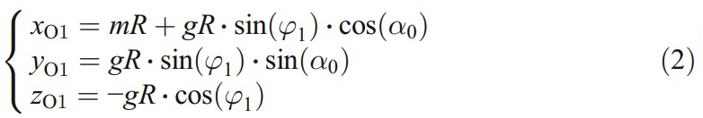
As indicated in Fig. 2, coordinate system XgYgZg represents the wheel frame while XYZ represents the stationary end mill frame. In this paper, the clearance is machined only after the helical groove has been ground, the cutter tip is located at coordinates (mR, 0, 0) and equations are expressed in the end mill frame.

Figure 3 shows the transformation procedures of wheel coordinate system for flat clearance machining. Assume that the wheel coordinate system is coincident with the end mill coordinate XYZ at the beginning, coordinate system XgY gZ g can be deduced by two translation parameters mR and -gR from O along X-axis and Z-axis, respectively. Rotating the frame XgY gZ g by an angle α0 about its Zg-axis (get the coordinate system Xg1Y g1Z g1), flat clearance angle with a value of α0 could be machined. In order to avoid the phenomenon of grinding burn, which is caused by too much contact area between wheel and clearance, the wheel is then rotated to the coordinate system Xg2Y g2Z g2 by an angle φ1 (Fig. 3). Now, the initial wheel position relative to the end mill is obtained. The wheel orientation can be expressed by the following vector:

and the wheel location can be expressed by

4. Eccentric clearance machining process

4.1 Machining principle

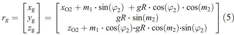
According to the wheel position provided in Fig. 1b, coordinates are built to express the initial positions of wheels to start the machining process (Fig. 4). The parameter φ2 is the rotational angle of the wheel frame about its Xg-axis. The wheel orientation can be given by the vector

and the wheel location can be expressed as

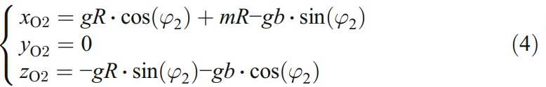
Figure 5a gives the wheel position relative to the end mill in eccentric machining process. The machining result shows that two faces are ground after the grinding process: one is the clearance face enveloped by the cylindrical face of wheel and the other is the unwanted face produced by the wheel circumference. Figure 5b shows the machining result based on Fig. 1b (i.e., the point p4 is coincident with point Q and gb= 10 mm). P1 is the intersection point of contact line and end mill contour. P2 is the intersection point of contact line and the wheel circumference. P3 is the intersection point of end mill contour and the wheel circumference.

Fig. 1 Machining process of clearance with flat, eccentric, and convex shapes

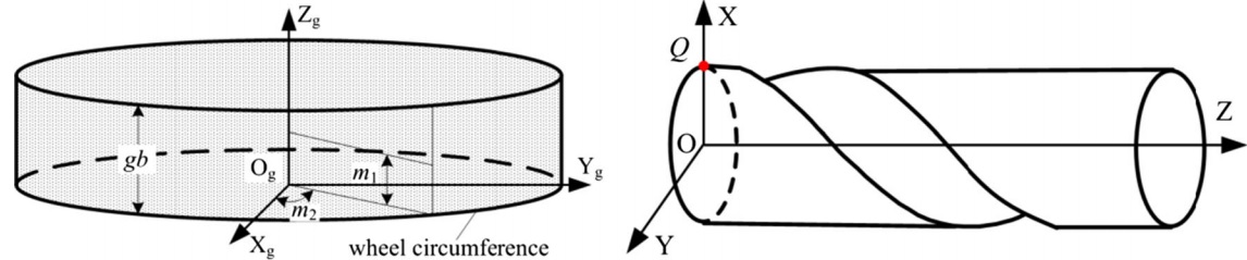
Fig. 2 Coordinates for wheel and end mill calculation. (a) Wheel coordinate. (b) End mill coordinate

Obviously, two problems can be observed from the figure: the envelope surface boundary (i.e., the clearance face boundary) is not coincided with the cutting edge and the unwanted machining face will affect other teeth when Φ’>Φ. Besides, the inclination angle φ2 and clearance angle α0 could not be calculated so far. To solve these three problems, further study is detailed in the following sections.

Fig. 3 Transformation procedures of wheel coordinate systems for flat clearance machining

4.2 Analysis of clearance face boundary

From Fig. 5b, it is learned that the envelope surface boundary will overlap with the cutting edge, as long as the point p1 is located on the cutting edge. Based on Eqs. (3) and (4), the cylinder face of the wheel as shown in Fig. 4 can be represented in this form by

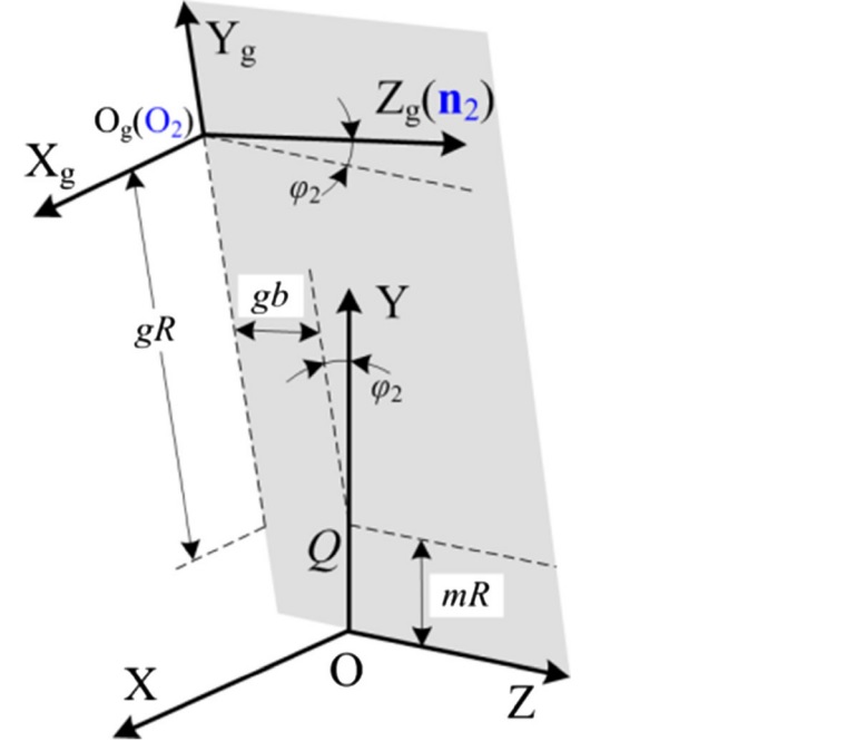
Fig. 4 Transformation procedures of wheel coordinate system for eccentric clearance machining

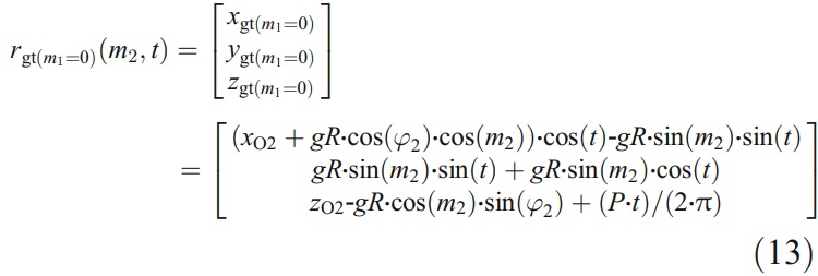
Then, a family of wheel surfaces can be obtained by moving the wheel along the cutting edge with a constant lead P and expressed as

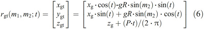
where t represents the rotation angle that the wheel moves around the end mill axis. According to the principle of envelope, the fundamental relationship for the clearance machining is formed as

(∂rgt/∂m1,∂rgt/∂m2,∂rgt/∂t)=0

Where

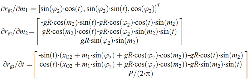
It can be simply denoted as

Or

Now, the envelope equation derived from the grinding process is expressed as Eq. (7), where m1∈[0, gb] and m2∈[0, 2π].

Fig. 5 Eccentric clearance machining mechanism. (a) Eccentric clearance machining process. (b) Contact lines of eccentric clearance machining

Substituting Eq. (8) and t=0 into Eq. (6), the contact line (i.e., line p1p2) of the wheel and the clearance at the initial processing position is obtained in the form

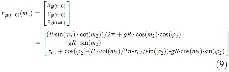
Finally, the coordinates of p1 (xp1,yp1,zp1) could be calculated by solving the equation x 2 gt(t=0)+y 2 gt(t=0)=mR2 . In order to make the envelope surface boundary coincide with the cutting edge, the point p1 must be moved to point p4 at the beginning (i.e., t=0 and point p4 coincides with point Q). Therefore, before the machining process, the wheel should

Table 1 Process parameters of eccentric clearance manufacturing

rotate and moves along the Z-axis from the frame XgYgZg (as shown in Fig. 4) with an angle λ and a displacement |zp1|. Where, λ is the angle between X-axis and the projection line of Op1 on the cross section of end mill, which can be shown as

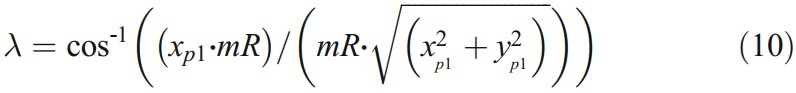
Table 2 Points on the contact line

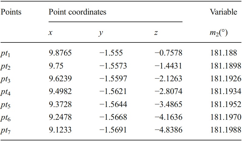
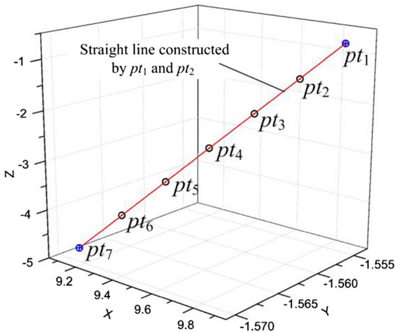
Fig. 6 Points on the contact line pt1pt2

4.3 Definition of the inclination angle

Substituting parameters listed in Table 1 into Eq. (9), the points on the contact line could be calculated. The results are shown in Table 2. Figure 6 shows the positions of points in a three-dimensional coordinate. Connecting the first and last point (pt1 and pt7) with a straight line, it is found that all of the other points lie in the line, which means that the contact line is also a straight line.

According to Fig. 5b, the relationship between φ2 and α0 is expressed in Figs. 7, and the following equations are concluded:

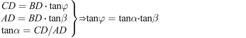
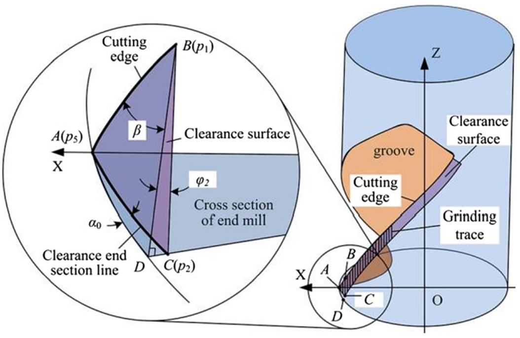
Fig. 7 Relationship between the clearance angle (α0) and the install angle (φ2)

from which it can be easily shown that

This equation shows that the inclination angle φ2 only depends on the helical angle β and the clearance angle α0.

4.4 Noninterference conditions

It is obvious that only when the angle Φ’ is smaller than Φ will clearance be machined without interference. From Fig. 5b, we learn that the angle Φ’ is produced by line p1p2 and line p2p3 on the cross section of end mill. So, the calculation of the angle Φ’ is divided into two parts in the next studies.

①Analysis of surface produced by line p1p2 Substituting zgt=0 into Eq. (6), a relationship can be deduced as

Now, by substituting Eqs. (8) and (12) into Eq. (6), equation of the machined contour (p2p5 in Fig. 5b) produced by line p1p2 on the cross section of end mill is obtained. Then, the coordinates (xp5,yp5,0) of point p5 could be calculated through solving equations of machined and end mill contours.

②Analysis of surface produced by line p2p3 Substituting m1=0 into Eq. (6), the helical surface generated by the wheel circumference moving along the cutting edge is obtained in the form

Fig. 8 Simulation of clearance machining process

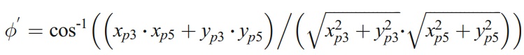
By solving the equation zgt(m1=0)=0, a function t= f2(m2) can be derived. Substituting it into Eq. (13), equation of the machined contour produced by line p2p3 on the cross section of end mill is obtained. Now, the coordinates (xp3,yp3,0) of point p3 are deduced. Based on the coordinates of point p5 and p3, the angle Φ’ can be expressed as

③Simplification algorithm

The approach mentioned above could obtain a precise value of Φ’, but the calculate process is very complicated. As the angle Φ’ do not influence the clearance geometry, a rapid evaluation method whose solution may have a permissible error will be more utility in practice.

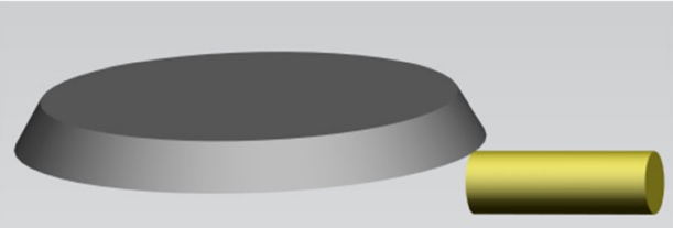
Fig. 9 Initial position of wheel for flat clearance machining

Fig. 10 Simulation result of flat clearance machining

Based on Fig. 7, the machined contour produced by line p1p2 on the cross section of end mill can be expressed as a segment of circular arc SAD, which is defined as

sAD = BD⋅tanβ = gb⋅cos (φ2) ⋅tanβ

According to Fig. 5b, the machined contour produced by line p2p3 can be approximately represented in the form

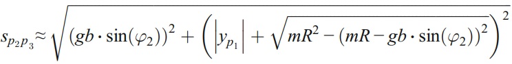
Now, the angle Φ’ can be given by

Considering that mR, β, and φ2 are parameters of end mill which could not be changed, the wheel thickness gb is the only variable to reach the noninterference condition: Φ’<Φ.

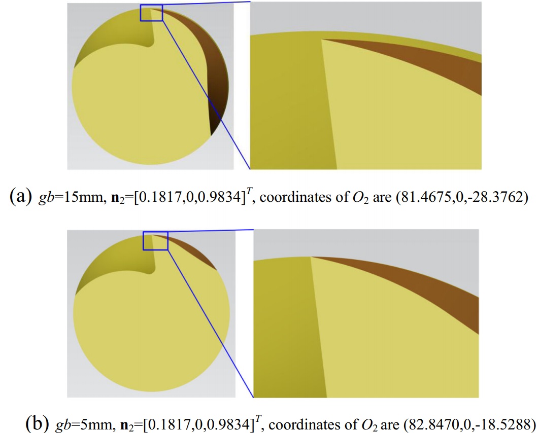
Fig. 12 Simulation result of eccentric clearance machining. a gb=15 mm, n2=[0.1817,0,0.9834]T, coordinates of O2 are (81.4675,0,–28.3762). b gb= 5 mm, n2=[0.1817,0,0.9834]T , coordinates of O2 are (82.8470,0,–18.5288)

5. Convex clearance machining process

As shown in Fig. 1c, the wheel orientation used to machine the convex clearance is easily obtained in the form

n3 = [0, 0, 1] T

and origin of the wheel frame is located at coordinates (xo3,yo3,zo3)

Fig. 13 Initial position of wheel for convex clearance machining

6. Examples

In order to verify the mathematical models established above, a clearance grinding simulation system is established by the UG secondary development technology. In the simulation, just like the actual grinding process, the wheel moves along a helical line (i.e., the helical cutting edge) step by step. Each step takes a Boolean subtraction operation: wheel as the “cutter” and blank as the “objective”. Then, the clearance model could be established by these Boolean operations (Fig. 8).

End mills with parameters of mR=10 m, p=60 mm, and α0=10° are taken as examples to verify the mathematical models. The wheels used in the examples have a radius of 75 mm

Fig. 14 Simulation result of convex clearance machining

6.1 Example of flat clearance machining

Substituting φ1=2° into Eqs. (1) and (2), the wheel orientation could be calculated as n1=[0.98,0.17,0.03]T , and coordinates of O1 are (12.58,0.45,–74.95). The simulation process is shown in Fig. 9 and the result is presented in Fig. 10.

6.2 Example of eccentric clearance machining

Based on Eq. (11), the inclination angle (φ2) of wheel used to machine the eccentric clearance can be deduced as 10.4675°. Fig. 11 provides the simulation process.

By substituting gb=15 mm into Eqs. (3) and (4), the wheel position parameters could be calculated as n2= [0.1817,0,0.9834]T and coordinates of O2 are (81.4675,0,–28.3762). According to Eq. (14), the angle Φ’ (Fig. 5b) can be calculated as 142.53°. The simulation result is shown in Fig. 12a. Obviously, interference will be occurred when Φ<Φ’ (i.e., end mills with more than four teeth could not be machined correctly). Besides, the cutting edge is overcutted, for it is inconsistent with the envelope surface boundary.

Based on Eq. (9) and (10), coordinates of p1 are deduced as (9.8784,–1.5550,–0.7476) and λ is equal to 8.9458°. Rotating and moving the wheel along the Z-axis from frame XgYgZg (as shown in Fig. 4) with 8.9458° and 0.7476 mm, and reducing gb from 15 to 5 mm, a new simulation result can be obtained (Fig. 12b). Now, a clearance could be ground properly as long as the adjacent cutter angle Φ is larger than 62.39° (because Φ’=62.39°).

6.3 Examples of convex clearance machining

Based on Eq. (15), coordinates of O3 can be calculated as (81.4675,0,–28.3762). The simulation process and result are shown in Fig. 13 and Fig. 14.

7. Conclusions

Based on the practical processes analysis, mathematical models for machining flat, eccentric, and convex shapes of clearance are established. Wheel orientations and locations are calculated and conditions to machine a desired clearance are discussed. Furthermore, a simulation system is developed to verify the mathematical models and visualize the machining process. The main conclusions are summarized as follows:

1. Examples show that mathematical models of clearance machining have been derived correctly.
2. For eccentric clearance machining, undercutting problems on the adjacent cutting edge can be solved by reducing the thickness of wheel. Furthermore, to machine a desired eccentric clearance, the envelope surface boundary should be coincided with the cutting edge, which leads to additional transformations for the wheel before starting the process.
3. Clearances obtained from the simulation program are solid models, which could be used as an input model for FEM analysis.

Acknowledgment

It is a project supported by the Important National Science & Technology Specific Projects (No.2012ZX04003-021) and “Taishan Scholar Program Foundation of Shandong”.