Development of analytical solid carbide end mill deflection and dynamics models
2020-06-29
Abstract
Accurate knowledge of machine dynamics is required for predicting stability and precision in a machining process. Frequency response function (FRF) measurements need to be performed to identify the dynamics of the systems experimentally. This can be very time consuming considering the number of tool-tool holder combinations in a production facility. In this paper, methods for modelling dynamics of milling tool is presented. Static and dynamic analysis of tools with different geometry and material are carried out by Finite Element Analysis (FEA). Some practical equations are developed to predict the static and dynamic properties of tools. Receptance coupling and substructuring analyses are used to combine the dynamics of individual component dynamics. In this analysis, experimental or analytic FRFs for the individual components are used to predict the final assembly’s dynamic response. The critical point in this analysis is to identify the interface stiffness and damping between the end mill and tool holder. The effects of changes in end mill parameters and clamping conditions are evaluated. The predictions are verified by measurements.
Introduction
Static and dynamic deformations of machine tool, tool holder and cutting tool play an important role in tolerance integrity and stability in a machining process affecting part quality and productivity. Excessive static deflection may cause tolerance violations whereas chatter vibrations result in poor surface finish. Cutting force, surface finish and cutting stability models can be used to predict and overcome these problems. This would require static and dynamic data for the structures involved in a machining system. Considering great variety of machine tool configurations, tool holder and cutting tool geometries, analysis of every case can be quite time consuming and unpractical. These data are usually obtained by testing using stiffness measurements and modal analysis. In this study, generalized equations are presented which can be used for predicting the static and dynamic properties of milling system components. Due to its wide use in industry, milling process is considered, however the same methods can be applied to other machining operations as well.
Modeling of milling process has been the subject of many studies some of which are summarized by Smith and Tlusty. The focus of these studies has mostly been on the modeling of cutting geometry and force, stability and prediction of part quality. The mechanistic approach has been widely used for the force predictions and also has been extended to predict associated machine component deflections or surface geometrical errors. An alternative method is to use mechanics of cutting approach in determining milling force coefficients as used by Armarego et al. Another major limitation on productivity and surface quality in milling is the chatter vibrations which develop due to dynamic interactions between the cutting tool and workpiece, and result in poor surface finish and reduced end mill life. Tlusty and Tobias identified the most powerful source of self-excitation which is associated with the structural dynamics of the machine tool and the feedback between the subsequent cuts on the same cutting surface resulting in regeneration of waviness on the cutting surfaces. In the early milling stability analysis, Tlusty used an approximate analytical model and time domain simulations for predicting of chatter stability in milling. Minis et al. used Floquet's theorem and the Fourier series for the formulation of the milling stability, and numerically solved it using the Nyquist criterion. Budak developed a stability method which leads to analytical determination of stability limits. The stability of low radial immersion milling has been investigated and modeled in where cases for doubled number of stability lobes are presented. These methods can be used to generate stability diagrams from which stable cutting conditions, and spindle speeds resulting in much higher stability can be determined for given work material, end mill geometry and transfer functions.
Demonstrations of cutting model implementation in CAD/CAM systems have been done in several studies. Altintas and Spence and Yazar et al. demonstrated that force models could be used to predict form errors and optimize feedrates based on simulation at the CAD/CAM stage. Weck et al. demonstrated determination of chatter free milling conditions in a commercial CAD/CAM software. Cutting force coefficients and end mill dynamics were needed for these simulations, which were determined experimentally. Generation of an orthogonal cutting database for a work material as Budak et al. did reduces the amount of experiments, and thus makes implementation of force models in CAD/CAM more practical. There is a need for more practical determination of structural properties of the cutting tool for a virtual machining system. Kops et al. determined an equivalent diameter for end mill based on FEA in order to be able to use beam equations for deflection calculations, which eliminate stiffness measurements for each end mill. Schmitz used substructuring methods to predict the dynamics of tool holder-end mill assembly using beam component modes.
In this paper, a precise modeling of end mill structure is presented for accurate determination of form errors and stability limits. End mill geometry is very complicated, thus in general, beam approximations do not provide accurate stiffness and transfer function predictions. Both FEA and analytical methods have been used for static and dynamic analysis of end mills. Simplified, but accurate equations are presented for end mills, which can be used in CAD/CAM systems for form error and stability limit calculations. The results are verified experimentally.
Nomenclature
A / Area (mm2)
D / Diameter (mm)
E / Modulus of elasticity (MPa)
F / Applied Force (N)
I / Second moment of inertia (mm4)
L / Length (mm)
Gmn / Assembly receptance FRF element
Hmn / Individual receptance FRF element
C / Viscous damping coefficient (Ns/m).
k / Stiffness (N/m)
ω/ Frequency (Hz)
ρ / Density (kg/m3)
fd / Flute depth
R, S / Mode shapes
kx, kθ / Linear and rotational connection stiffness
cx, cq / Linear and rotational connection damping
Subscripts
m / Coordinate
n / Location of the force
n / Location of the force
1. Static analysis of the end mill
The tool holder is assumed to be rigid and the cantilever beam model is used for static analysis of end mills. The main objective of the static analysis is to determine the deflection along the end mill axis for given geometry and loading. The loading and boundary conditions of the end mill used in the model are shown in Fig. 1, where D1 is the mill diameter, D2 is the shank diameter, L1 is the flute length, L2 is the overall length, F is the point load, I1 is the moment of inertia of the part with flute and I2 is the moment of inertia of the part without flute.
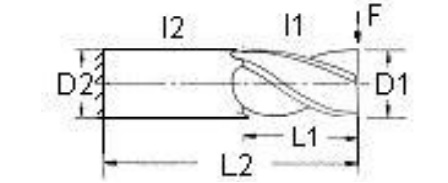
Figure 1. Loading and boundary conditions of the end mill
The moment-area theorems are used to determine the maximum deflection at the end of the cutting tool.

1.1 Moment of Inertia
For analytical formulation, models of 4-flute, 3-flute and 2- flute end mills are used to determine the moment of inertias. Due the complexity of the cutter cross-section along its axis, the inertia calculation is the most difficult aspect of the static analysis. The cross sections of the end mills are as shown in Fig. 2.
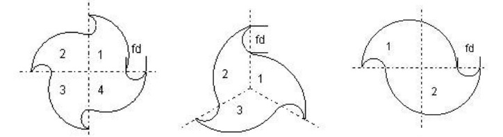
Figure 2. Cross sections of the 4-flute, 3-flute and 2-flute end mills
In order to determine the inertia of the whole cross section, inertia of region 1 is first derived, and inertia of the other regions are obtained by transformation. The total inertia of the cross section is then obtained by summing the inertia of all regions. The effect of the arcs due to flute depths (fd) is added to total inertia. Regions for 4-flute, 3- flute and 2-flute are shown in Fig. 3.
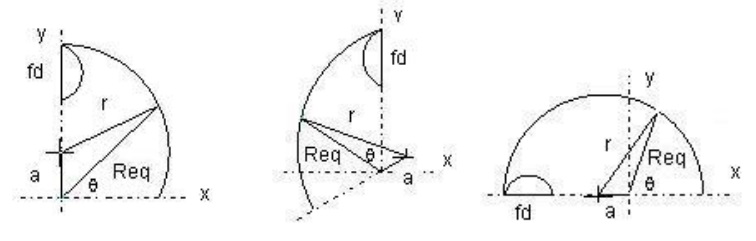
Figure 3. Region 1 of 4-flute, 3-flute and 2-flute end mill
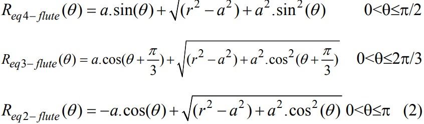
The inertia of region 1 is derived by computing equivalent radius Req in terms of the radius r of the arc, position of the center of the arc (a) and θ. Using cosine law the equivalent radius Req for region 1 of 4-flute, 3-flute and 2-flute end mill with respect to x- and y-axes as:
The moment of inertia of region 1 of a 4-Flute end mill about x- and y- axes can be written as:
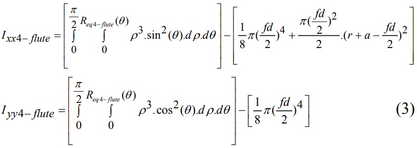
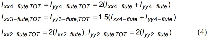
where 0<ρ≤Req(θ). The same formulation can be written for region 1 of the 3-flute and 2-flute end mill. After transforming the inertia of region 1, the total inertias are found as follows:
1.2 FE Modeling and Analysis of Cantilever Tool
For parametric and geometric solid modeling, FE modeling and analysis, I-DEAS® is used. Many simulations were performed for end mills with different material, flute diameter, shank diameter, flute length, overall length and number of teeth. Modulus of elasticity and density are 200 GPa and 605 GPa,, and 8600 kg/m3 and 12500 kg/m3 for HSS and carbide end mills, respectively. The Poisson’s ratio is 0.3 for both of the tool materials.
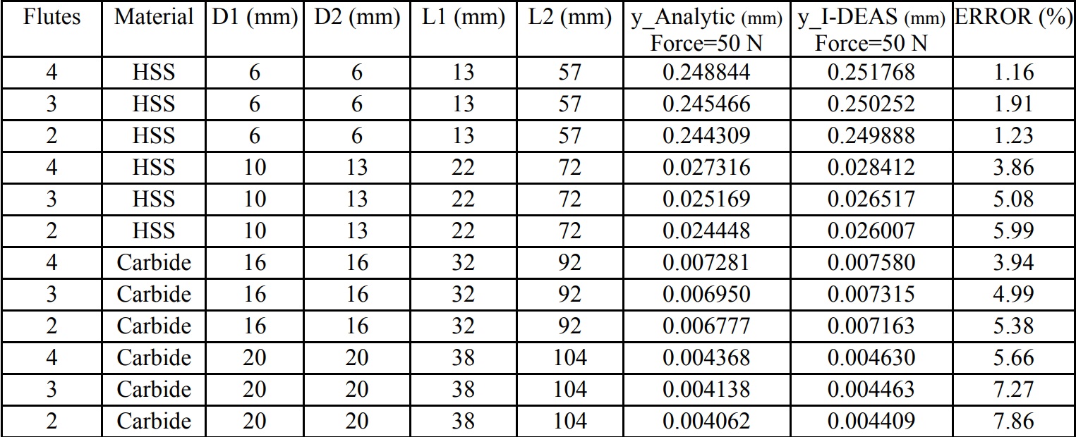
FE method is used to determine deformations of the end mill when a point force is applied at its end. An example of end mill deflection is shown in Fig. 4. FEA is applied to great variety of end mill geometries in I-DEAS®. The comparison of some deflections by analytical solutions and I-DEAS® are shown in Table 1. Approximately sixty end mills were tested.
Modeling and FEA can be unpractical and time consuming for each end mill configuration in a virtual machining environment. Therefore, simplified equations are created to predict deflections of end mills for given geometric parameters and density.
Table 1. Results of the analytic equations and I-DEAS analysis
The static characteristics of end mills can easily be determined by analytic equations. After the comparison of analytical and FEA results, the corrected deflection equation has the following form:

where Yanalytic is in mm. The constant C is 0.984, 0.985 and 0.986 and N is 0.983, 0.981 and 0.980 for 4-Flute, 3-Flute and 2-Flute cutters, respectively. The error in this approximation is less than % 1. In the analytical deformation equations, the evaluation of the integral formulas is very complex. It is possible to determine the maximum deflection of the end mill using:
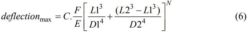
where F is the applied force and E is the modulus of elasticity (MPa) of the end mill material. The geometric properties of the end mill are in mm. The constant C is 9.05, 8.30 and 7.93 and N is 0.950, 0.965 and 0.974 for 4-Flute, 3-Flute and 2-Flute cutters, respectively. The error in this approximation is less than 5%.
4-flute high speed steel long slender end mill is selected to demonstrate the accuracy of analytical results. The mill and shank diameter is 6 mm, the flute length is 38 mm and the gauge length is 75 mm. A force is applied to end point of the end mill and measured by dynamometer and displacements at the two points of the end mill are measured by dial gage. Total displacement of the end mill is equal to summation of clamping displacement, beam displacement and rotational displacement. Rotational displacement is assumed to be zero. The experimental beam stiffness is 75 N/mm and the stiffness of the end mill, which is calculated by using analytical equation, is 70.5 N/mm. The agreement between two stiffness values is very satisfactory.
2. Dynamic analysis of the end mill
2.1 Flexible End mill – Rigid Holder
2.1.1 Analytical Model
Dynamic analysis is used to determine mode shapes and natural frequencies of the cutting tool structures. A modeling method for transverse vibrations of an end mill is developed. End mill is a segmented beam, one segment for the part with flute and the other segment for the shank. The beam model with two different geometric segments is shown in Fig. 5.
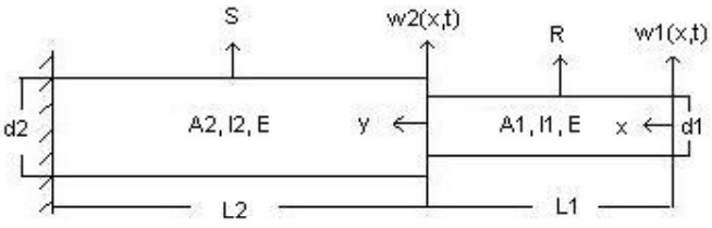
Figure 5: The geometry of the beam with two different geometric segments
where I1, I2 and A1, A2 are the moment of inertias and the areas of the segments, respectively. R(x) and S(y) are the mode shapes, and w1(x, t) and w2(x, t) are the displacement functions. The governing equations of motion, neglecting the rotational inertia and shear formation, can be converted into the well-known Euler-Bernoulli equations:
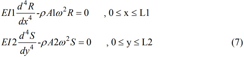
where E is the modulus of elasticity and ρ is the density. The solution of Eq. (8) can be expressed as:
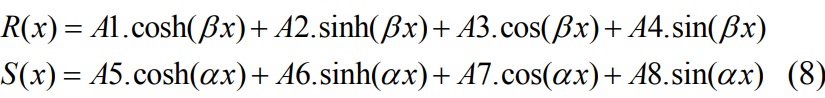
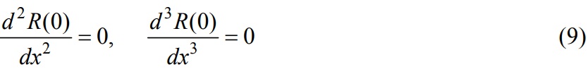
where A1, A2, A3, A4, A5, A6, A7 and A8 are arbitrary constants. It is necessary to accompany the general solutions with the boundary conditions. The boundary conditions are as follows. At x=0 (i.e. at the free end), bending moment and shear force are defined as:
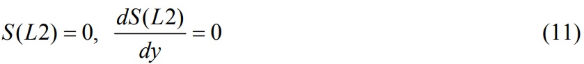
At x=L1 and y=0 the continuity equations for displacement, slope, moment and shear force are as follows:
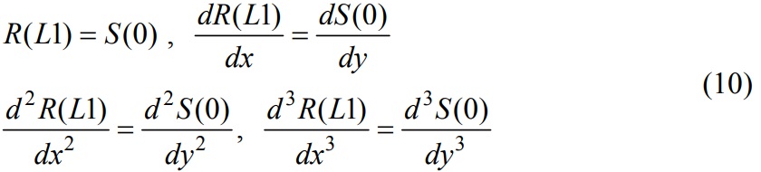
At y=L2 (i.e. at the fixed end) displacement and slope equations:
These 8 conditions defined by equations (9-11) are sufficient to solve for the 8 arbitrary constants. The equations involving these constants can be written in the following form:
[C]{A}=0
where Aj is the vector of the 8 arbitrary constants and the coefficient matrix [C] is of dimension (8 x 8), and is given by:
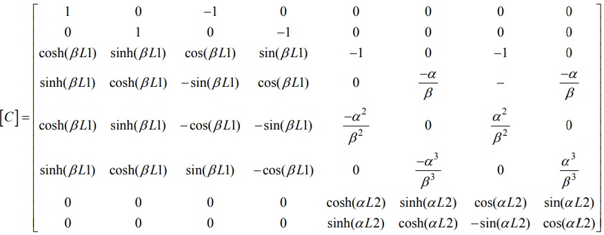
The characteristic equation is determined if |C|=0.The natural frequencies are computed from the solution of characteristic equation as:
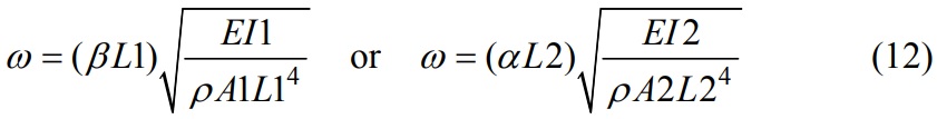
The mode shapes according to the frequencies are obtained by combining R(x) and S(y) from Eq. (8).
2.1.2 FE Modeling and Analysis of Cantilever End mill
In I-DEAS®, models are built to define geometry, material properties, element types and constraints for end mills. Natural frequencies and mode shapes are obtained using FEA. Many end mills with different material and geometric parameters are analyzed. As an example, natural frequencies and mode shapes of an end mill with 4-Flute, 10 mm diameter, 68 mm overall length and 22 mm flute length are shown in Fig. 6.
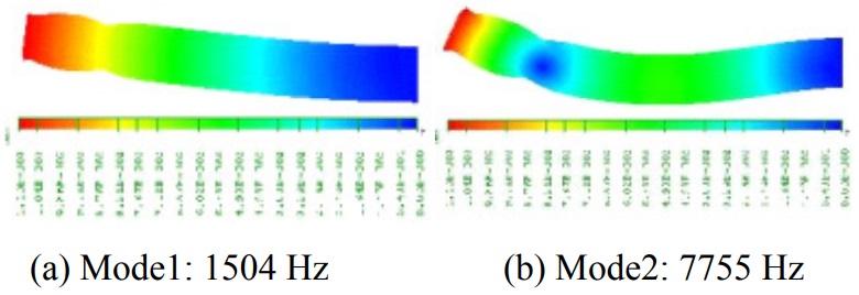
Figure 6. Example of natural frequencies and mode shapes of an end mill
The lateral and vertical bending frequencies are different for 2-flute cutter. The cross section of the 2-flute cutter is not symmetric with respect to x and y axes, so the moment of inertia Ixx and Iyy are different.
As the end mill length/diameter ratio increases, the natural frequency of the end mill decreases (Fig. 7). 2-flute cutters have the greatest natural frequency and 4-flute cutters have the least because of the cross section. The carbide end mill s have higher natural frequency than HSS end mills because of their high modulus of elasticity (Fig. 8).
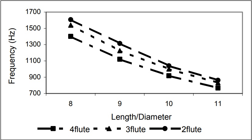
Figure 7. Relationship between natural frequencies (Mode1) of HSS end mill and end mill length/diameter ratio
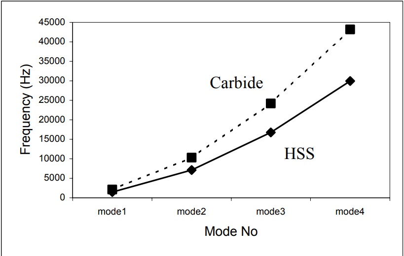
Figure 8. Comparison between Carbide and HSS natural frequencies
2.2 End mill Dynamics Including Machine Flexibility
2.2.1 Receptance Coupling Substructure Analysis for End mill Dynamics
Complete machine structure is divided into two parts, end mill and tool holder/spindle. The description of the assembly model and the connection parameters are shown in Fig. 9. The four connection parameters (linear and torsional springs and dampers) must be determined to predict end mill point frequency response function (FRF). According to these parameters, end mill and tool holder/spindle FRFs are coupled using receptance coupling substructure analysis (RCSA). RCSA is a very efficient method to predict dynamic response of end mills without measurements for each end mill, tool holder and spindle combination. In this study, the analytical model developed for the end mill dynamics given in section 2 is used together with RCSA to determine the total dynamics of the machine.
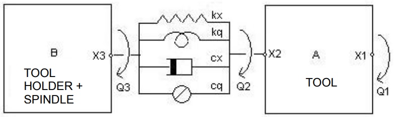
Figure 9. End mill and tool holder/spindle assembly
In RCSA, each component of the assembly must be tested separately to determine the component FRFs. Nevertheless, this is only possible if the impact tests on the individual parts provide enough information to predict accurately the dynamic properties of the assembled structure. In case of low natural frequency modes, the dynamics at the end mill and tool holder/spindle interface might not be adequately represented in the modal data. Furthermore, in many cases the measurement of component dynamics is not practical which is the case for free-free end mill.
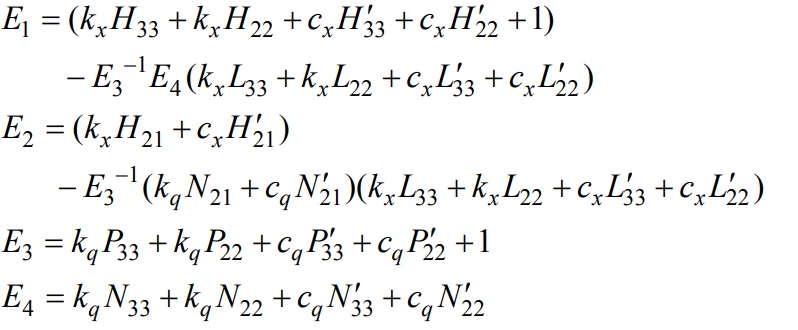
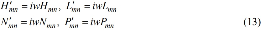
The direct and cross free-free FRFs of the end mill are calculated analytically using the model presented in this paper. In the formulation, the component modes are represented by H whereas G is for the assembly FRFs. Direct and cross deflection receptance terms (H11, H22 and H12= - H21), displacement under applied force (Lmn), rotation under applied force (Nmn) and the rotation under applied moment (Pmn) for the component A are derived analytically. For the calculations, density (ρ), elastic modulus (E), viscous damping coefficient (c) and second moment of inertia (I) are required. In the static analysis section, an analytic equation for the maximum displacement at the end mill tip was derived (Eq. (1)) which can be used to determine the stiffness of the end mill. The effective diameter of the end mill and the second moment of inertia can be calculated using the analytical equations developed in section 1 for segmented beam with different moments of inertias and the cantilever beam equation of the uniform cylinder. The mass of the end mill can then be determined using the natural frequency and stiffness both from analytic equations. The damping ratios for many HSS and carbide end mills have been determined experimentally. Average values of ζ=0.018 and ζ=0.012 have been obtained from experimental data for HSS and carbide end mills, respectively. By using these dynamic properties, approximate c values are estimated. Note that c values determined this way includes the damping of the end mill only as they are identified from end mill’s component mode dynamics. These damping ratio values can then be used in the analysis of different end mills.
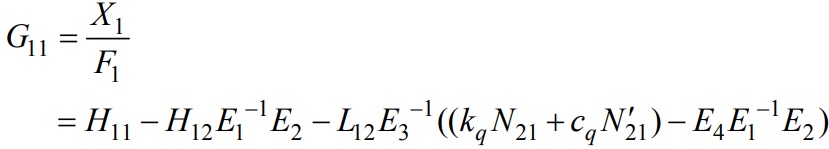
where
2.2.2 Identification of Connection Parameters
In experiments, the end mill point FRFs (G11) of the end mill/tool holder/spindle assembly are measured for different end mills. The connection parameters (kx, kq, cx, cq) are determined using lsqnonlin command of Matlab Optimization Toolbox. Isqnonlin solves nonlinear least squares problems, including nonlinear data fitting. X=lsqnonlin (fnctn,Xo) starts at a point X0 and finds a minimum to the sum of squares of the functions described in fnctn. Our syntax is [X, resnorm, residual, exitflag, output]=lsqnonlin(fnctn,X0,lb,ub,options]. The solution is always in the range lb <= X <= ub. The optimization parameters (max iteration number, max function evaluation number, tolerances for function and X values) are specified in the structure options. The value of the residual for a solution X, the value exitflag (0,1) that describes the exit condition and the structure output that contains information about the optimization are returned. According to the calculated spring and damper parameters, the end mill point FRF of the assembly is predicted analytically using Eq. (13). The experimentally measured result and the predicted results for G11 are compared in the next section.
The knowledge of the FRF of the end mill point is used to predict the stability lobe diagrams. Unstable and stable regions can be determined depending on the spindle speed and axial depth of cut, b. The model parameters for each mode and the chatter frequencies around the natural frequency of the structure are used to simulate the stability lobes. The critical axial depth of cut can be seen easily from the stability lobes. Therefore, for a given end mill on a particular machining center, the stable milling conditions can be determined completely analytically. This is very useful information in a virtual machining environment, which is the next step for CAM.
The knowledge of the FRF of the end mill point is used to predict the stability lobe diagrams. Unstable and stable regions can be determined depending on the spindle speed and axial depth of cut, b. The model parameters for each mode and the chatter frequencies around the natural frequency of the structure are used to simulate the stability lobes. The critical axial depth of cut can be seen easily from the stability lobes. Therefore, for a given end mill on a particular machining center, the stable milling conditions can be determined completely analytically. This is very useful information in a virtual machining environment, which is the next step for CAM.
3. Experimental verification
3.1 End mill Deflection and Maximum Surface Error
Milling forces can be modeled for given cutting and cutter geometry, cutting conditions, and work material. The cutting forces in both directions can be used to determine milling tool deflections. In milling, the surface is generated when the cutting flutes intersect the finished surface. Thus, deflections of the end mill at those points are imprinted as surface form errors. The simulation of the surface form error in milling is given in.
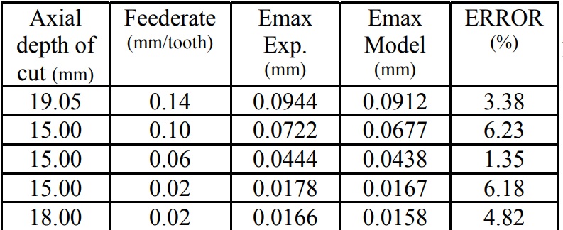
The stiffness of an end mill can be calculated using the analytic model. The stiffness values are used to predict the maximum surface error generated by the end mill. For surface error calculation, the cutting forces are determined according to work material properties, cutting and end mill conditions in by using milling force modeling. The results are verified using the experimental results in. 4-flute high speed steel end mill with 300 helix angle is used for the comparison. The end mill diameter is 19.05 mm and the end mill gauge length is 54.5 mm. The stiffness of this end mill is calculated as 12761 N/mm.
The model results agree with the experimental results (Table 6). The error in the prediction of the maximum surface error (Emax) is less than 6%.
Table 6. Experimental and calculated maximum surface error results
3.2 Flexible End mill and Rigid Holder/Spindle
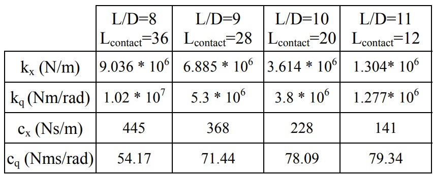
4-flute carbide end-mill with long overhang is selected to demonstrate the accuracy of analytical results. The mill and shank diameter is 8 mm, the flute length is 41 mm and the gauge length is 80 mm. FRF measurement was performed to determine the transfer function of the end mill which is shown in Fig. 15. Table 7 shows the identified frequency, stiffness, damping and mass values for the end mill. For comparison with analytical model predictions, the results obtained using the cylinder approximation for the end mill are also shown in Table 7 and Fig. 14. The cylinder with the same diameter and length is used in calculations. The graphs between the magnitude of the transfer function and frequency for all methods are shown in Fig. 15. Due to the long flute length of the end mill, the cylinder approximation is very poor in this case. The approximation results could be improved by using an effective diameter for the cylinder. As the end mills do not have circular cross sections along the flute length, the analytical solution is the most powerful approximation to find the dynamic properties. The model presented in this paper can be used to determine the dynamics of end mills for a given geometry, material and clamping conditions.
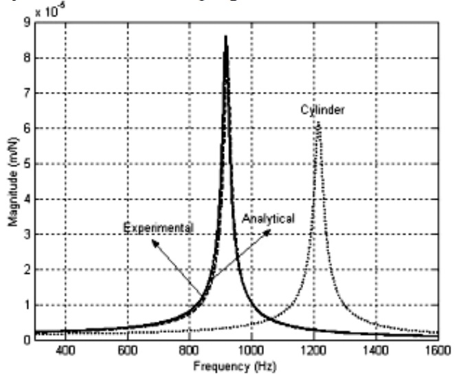
Figure 14. Magnitude of the transfer function for the experimental, I-DEAS, analytical and cylinder methods
Table 7. The comparison of the dynamic properties obtained from experimental, analytical and cylinder methods
3.3 Flexible End mill and Flexible Holder/Spindle
In this section, the FRFs using analytical models and the RCSA are compared with experimental results for verification. For the identification of the interface stiffness and damping between the end mill and tool holder, different end mill geometries, materials and clamping conditions are used. Contact parameters are identified and presented.
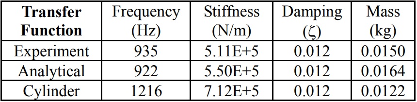
The tool holder/spindle direct FRF (H33) is measured at the free end in x/y directions by using low mass accelerometer and impact hammer. The measured FRF of the CAT40 tool holder/spindle is shown in Fig. 9. The same tool holder is used with different end mills, and therefore the same FRF (H33) is used in RCSA in the following examples.
The tool holder/spindle direct FRF (H33) is measured at the free end in x/y directions by using low mass accelerometer and impact hammer. The measured FRF of the CAT40 tool holder/spindle is shown in Fig. 9. The same tool holder is used with different end mills, and therefore the same FRF (H33) is used in RCSA in the following examples.
Figure 9. Measured FRF of tip of HSK40 tool holder/spindle combination
3.3.1 Experiment 1
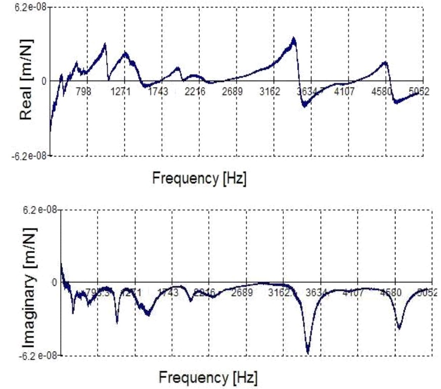
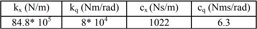
A carbide end mill with 4 flutes, 8 mm diameter, and 100 mm length is used for test. Different lengths (length to diameter ratios of 8:1, 9:1, 10:1, 11:1) are selected for the measurement.25 Nm clamping torque is applied on CAT40 holder. The end mill effective diameter and damping coefficient were determined as 7.49 mm and 5 Ns/m, respectively. After the nonlinear least square evaluation, the stiffness and damping coefficients are determined as shown in Table 2.
Table 2: Stiffness and damping coefficients for experiment 1
The measured and predicted FRFs using analytical component FRFs and RCSA are given for the shortest and longest end mills Fig. 10. The response is governed by only the first mode of the end mill, and thus only the first beam mode is used in the analytical component modes. As the contact length (Lcontact) that is in the tool holder decreases, natural frequency decreases and flexibility increases. All connection parameters except rotational damping increase, when Lcontact increases. The agreement between the experimental results and the predictions is satisfactory.
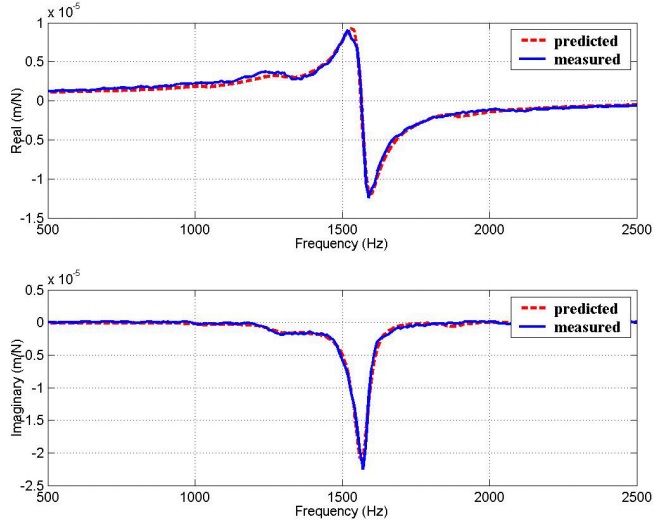
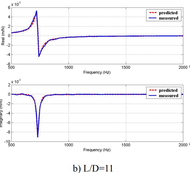
Figure 10. Predicted and measured FRFs for experiment 1
3.3.2 Experiment 2
In the experiment 2, the HSS end mill, which has 16 mm diameter, 85 mm overhang and 4 flute, was mounted in CAT40 tool holder. The effective diameter of the end mill and the damping ratio were determined as 15.56 mm and 20 Ns/m, respectively. The linear and rotational spring and damping coefficients for the connection between the end mill and tool holder/spindle are given in Table 3. The agreement between the predicted and measured results can be seen from the Fig. 11.
Table 3. Stiffness and damping coefficients for experiment 2
Because of the interaction between tool holder/spindle dynamics and the end mill dynamics, two close modes are experienced as shown in the figure. The tool holder/spindle mode at the approximately 1042 Hz and the cantilever end mill mode affect each other strongly resulting in 2 separate peaks. As a result, G11 is reduced which indicates that the tool holder/spindle is acting like a dynamic absorber for the end mill.
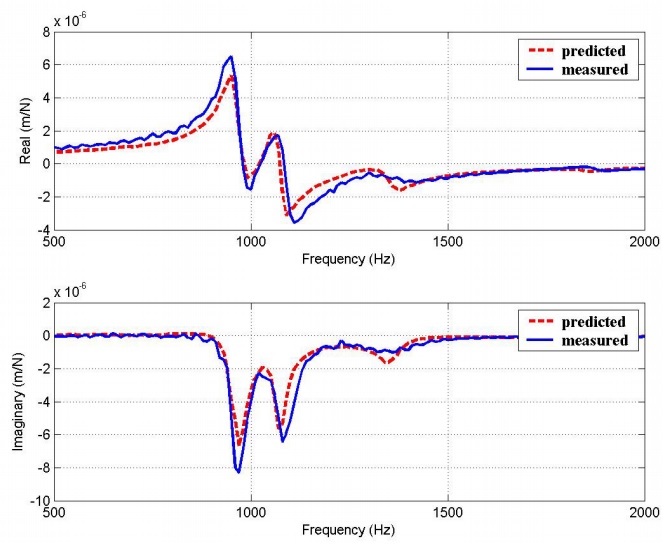
Figure 11. Predicted and measured FRFs for experiment 2
3.3.3 Experiment 3
HSS and carbide end mill with 4 flutes, 20 mm diameter, and 104 mm length are used for test. Different clamping torque values (25 Nm, 35 Nm and 45 Nm) are applied on CAT40 holder. The end mill effective diameter was determined as 19.498-mm. Damping coefficients for HSS and carbide tools were 26 Ns/m and 60 Ns/m, respectively. The nonlinear least square evaluation is used to find the stiffness and damping coefficients for HSS and carbide end mill and tool holder/spindle combination (Table 4). The stiffness and damping coefficients for the HSS end mill and tool holder pair are slightly less than connection coefficients for carbide tool and tool holder pair. As the clamping torque applied on tool holder is increased, all coefficients increase. These values can be used to predict the effect of the clamping torque on end mill dynamics and its stability.
Table 4 Stiffness and damping coefficients for experiment 3
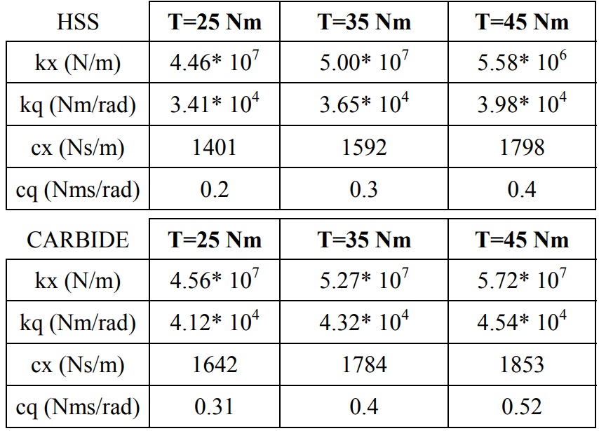
Figure 12 shows an example of the experimental and predicted direct end mill point FRFs (G11) for end mill material of HSS and carbide. The overall agreement between the predicted and measured results is good.
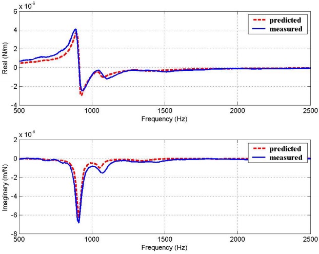
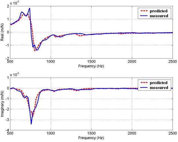
Figure 12. Predicted and measured FRFs for experiment 3
4. Conclusion
Dynamic and static properties of milling tools are very important for machining precision and chatter stability. In general, approximate analytical or experimental results are used to determine these characteristics. Approximate results do not provide accurate information particularly for the dynamics and chatter stability. Experimental methods, on the other hand, are time consuming considering the possible number of end mill and tool holder combinations, end mill geometry and material in an industrial setting. The analytical models presented in this work eliminate the need for transfer function measurements for every end mill assembly. The models consider the complex geometry of flutes in development of cross sectional properties. End mills have flutes and unfluted sections, which further complicate their geometry. This segmented characteristic has also been considered in static and dynamic modeling. RCSA model has been used for combining the measured dynamics of the tool holder/spindle and the analytically determined end mill modes. Both static and dynamic predictions are demonstrated to be extremely accurate for variety of cases. The approach presented here is very useful for implementation in a virtual machining system where the form errors and stability limits for a milling application can be determined automatically.