Study on the optimal feed rate for high speed machining
2020-04-24
Abstract
Conventional NC machining is the removal of material at a fixed rate of feed. Since the volume removed and the force on the tool are not fixed, the cutter is susceptible to bending due to heavy loads, which affects the accuracy and quality of the machining. In this paper, we first use the reverse displacement method to plan the tool path of medium machining and finishing, and then propose different methods of adjusting the feed rate for medium machining and finishing respectively; the mathematical relationship between the cutting force and the feed rate is used to adjust the feed rate during medium machining, so that the cutting force remains within the appropriate range, the load on the tool does not vary too much, and in finishing, the curvature of the surface is used to estimate the volume of each machining point, using the concept of equal volume removal rate, in order to improve the disadvantages of NC machining with a fixed feed rate, to optimize the feed rate.
I. Preface
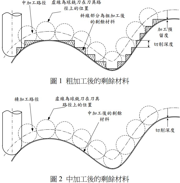
NC machining can generally be divided into rough machining, semi-roughing and finish machining, in which rough machining mostly uses iso-height machining to quickly remove the workpiece embryos in a straight and contoured toolpath to form a finished product prototype, resulting in a stepped residue, as shown in Figure 1, which will cause the cutting load of the tool in the intermediate machining to change too much, resulting in tool breakage or undercutting. If the feed rate is fixed in the conventional way, the removal volume of each CL point will be different and the cutting force will be different due to the different curvature of the curve. The methods of maintaining cutting forces within reasonable limits in the current literature can be broadly distinguished as follows.
1. Use the tool path to avoid excessive cutting force:
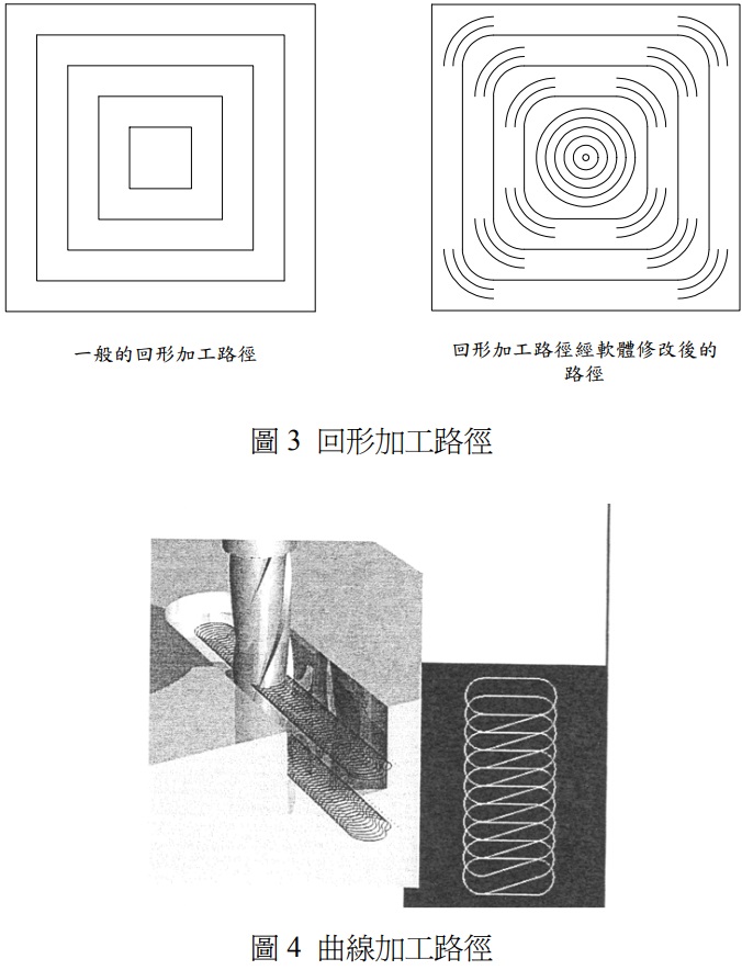
For example, the cutting path is carried out near the turning point to replace the right-angle path with a smooth path and the interpolation path to reduce the cutting force, as shown in Figure 3 [1]. In general, when conventional grooves are processed, the diameter of the milling cutter is used as the width of the groove and the cutting force is very high at this time.
2. Replacing the traditional linear approach with the curvilinear technique:
Relying on the different curvature of each process point in the curvilinear processing path, the concept of equal volume removal rate is used to derive the value of the controller's real-time interpolator (Real-time Interpolator), after calculating it with the curvilinear technique, as shown in Figure 4. Each position parameter corresponds to a different curvature and thus produces a different feed rate [3~6]. This method is very suitable for finishing where the machining path is a smooth curved pattern.This article differs from the above approach by using the concept of real machining volume removal rate with the cutting force to adjust the feed rate, so the cutting force will be maintained within a reasonable range. In this article, two different methods of automatic adjustment of the feed rate are proposed for medium machining and finishing machining, so that the cutting force does not vary too much during the machining process. When the tool removes more material volume, the feed rate is reduced, so that the cutting force decreases, the tool is not subject to too much load, machining accuracy and processing quality will be better; on the contrary, when the tool removes less material volume, the feed rate can be increased to increase processing efficiency.
II. Process route planning
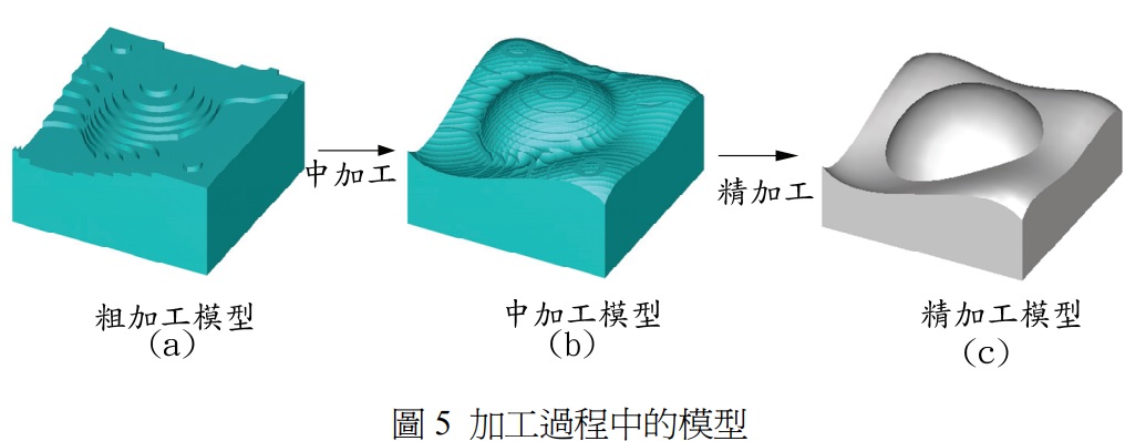
Before finishing, we must first remove the remaining volume of the stepped shape resulting from the coarse cutting, as shown in Figure 5 (a). The cutting path is to maintain a certain amount of finishing allowance along the surface of the surface to do the surface cutting, then machining, as shown in Figure 5 (b), and finally a finishing process to obtain a complete model, as shown in Figure 5 (c).
The approach taken in this paper for toolpath planning is to generate toolpaths by reverse displacement method and through point curves with step length and tool spacing (Step over) to find the appropriate CL point, with the following detailed steps.
1. Find the tool path by the reverse displacement method.
2. use the tool step length to find the appropriate CL point position.
3. Find the next tool path from the tool pitch value with the Z-map method.
2-1 Reverse displacement method
In this study, the method of reverse displacement is used to generate the control point of the tool path. As shown in Figure 6, the tool is first reversed and the center of the tool is kept on the surface. The center of the tool remains on the displacement surface during actual cutting, and the desired surface shape is obtained by cutting along the displacement surface. Taking a spherical end mill with radius R as an example, if { x(m), y(n), z’(m, n) } represents the coordinates of the CC point on the current model, then the height of the displaced surface at this location z'(m, n) can be obtained from the following equation [7].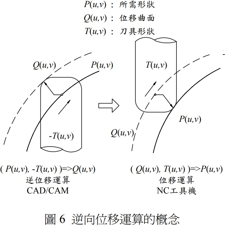
%E5%BC%8F.jpg)
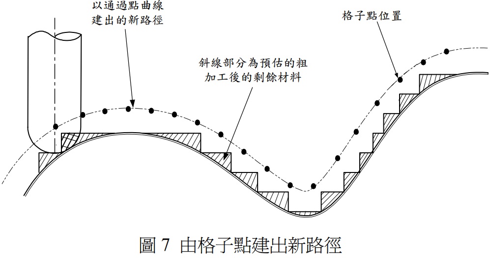
(1) The center position of the tool is the maximum value of "the sum of the surface height of the lattice points and the height of the tool surface" within the projection area of the tool. h(i,j,m,n:R) indicates the height of the tool surface at the lattice point position (i,j). When the grid point position is obtained, then connect all the grid points in the same column into a new curve with a pass-through point curve, as shown in Figure 7, which is the tool path.
2-2 Step length of the toolpath
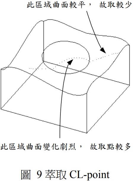
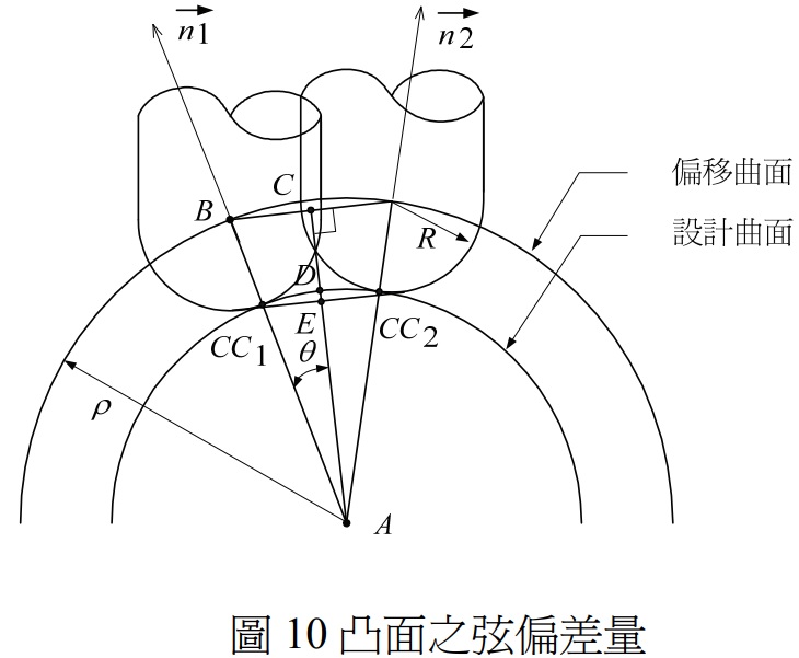
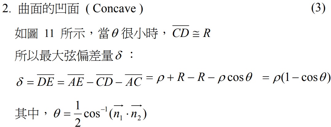
In NC machining, the tool is mostly cut in a straight line, and if the number of machining points is small, the surface of the machined surface will be rougher, and if the number of machining points is large, the surface of the machined workpiece will be smoother, but will take longer to plan ahead. So in order to achieve a balance between the surface roughness of the workpiece and the lead time, it is common to find a set of straight lines to approximate the curve and make the maximum chordal deviation smaller than the given machining margin, as shown in Figure 8. This algorithm avoids the phenomenon of excessive fetch points in flatter surfaces, as shown in Figure 9. The method of finding the maximum amount of string deviation can be divided into the following two conditions according to the surface's appearance characteristics.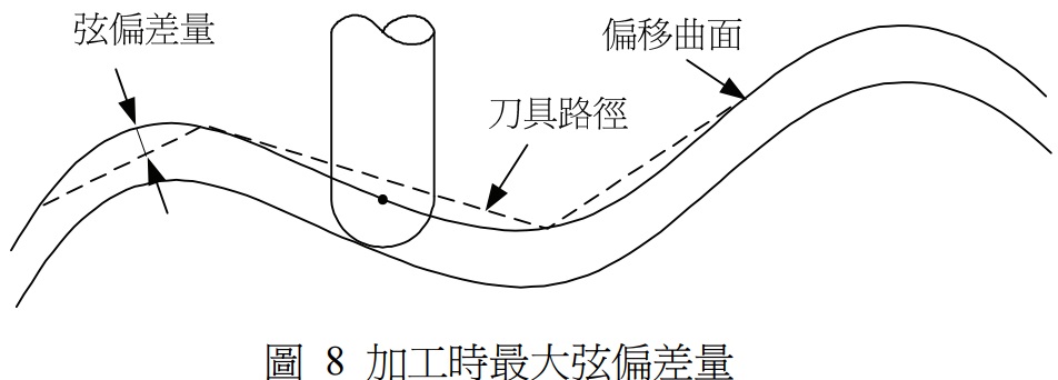
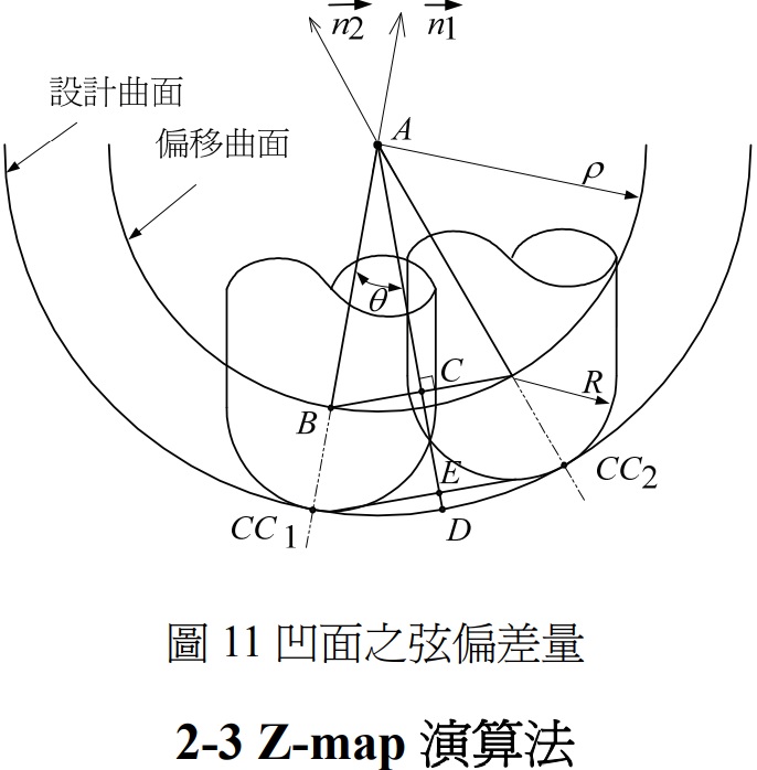
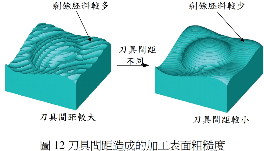
A workpiece machined with a larger tool pitch value will leave a layer of embryos between the adjacent cutting paths due to undercutting, called a scallop height, so by machining with a smaller tool pitch value, we can obtain a better machining surface accuracy, as shown in Figure 12.
In this paper, the tool spacing of the machining path is generated based on the grid points, but since the spacing of the grid points directly affects the machining error and the memory size required by the computer program, so this paper adopts Z-map theory [8] to generate accurate tool spacing, Z-map can solve the memory problem because it allocates memory by area planning, the detailed steps are as follows.
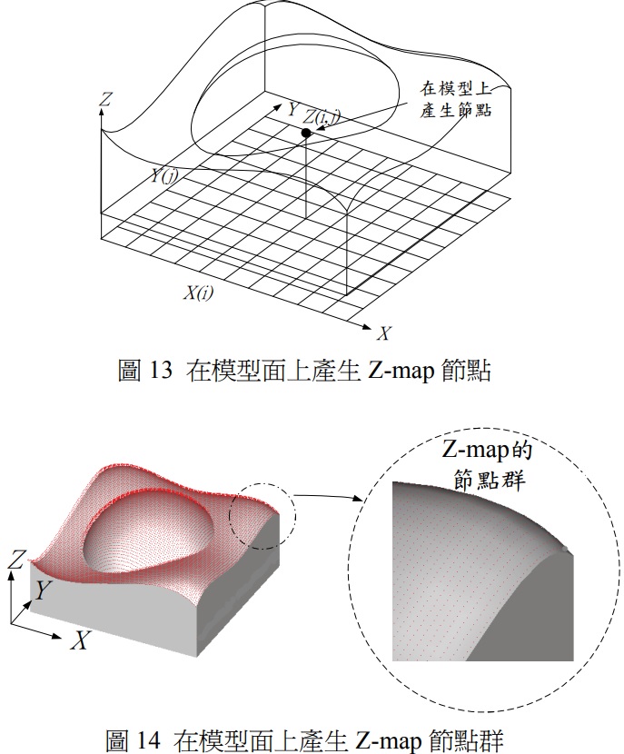
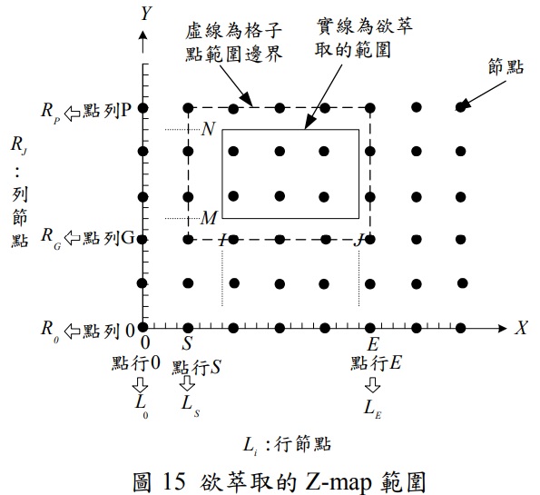
1. Generate node data on the model surface.
First, a group of nodes with the same interval distance are generated on the model surface, as shown in Figures 13 and 14.
2. Find the nodes on the displacement surface.
The node can be moved to a displacement surface using the reverse displacement method.
3. Z-map to extract grid point coordinates.
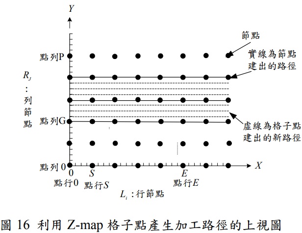
Take Fig. 15 as an example, to extract the height of the grid points from row I of column N to row J of column M, do the following:
(a) Find the location of the grid point range boundary:
(b) Check whether I, M falls on the dot row or dot column,
if so, set this dot row or dot column as the starting position of the grid point range boundary of I, M, if not, find the previous dot row or dot smaller than this position as the starting position of the grid point range boundary.
(c) Check whether J and N fall on a dotted row or column.
If yes, set this dot row or column to the end of the J, N grid dot range boundary; if no, find the next dot row or column larger than this position to the end of the grid dot range boundary.
(d) Extraction lattice point coordinates.
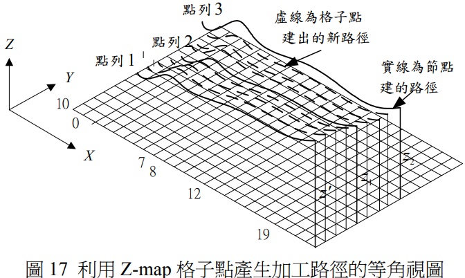
Having known the boundaries of this lattice point range, together with the known node coordinates, the following formula can be used to find all the lattice point coordinates in this rangeGrid point height = node height + distance × slope (4) where: slope = [(height of the previous node at the location of the grid point) - (height of the next node at the location of the grid point)] / (distance of the XY plane straight line between the two nodes) distance = number of grid points × distance between the grid points node height: height of the Z-axis at the previous node at the location of the grid point 4. Create a new path: create a new path by passing the grid points in the same column after Z-map through a point curve, as shown in Figure 16 and Figure 17.
III. Principle of adjusting the rate of feed to the process
As the cutting force is proportional to the volume of material removed by the tool, when the volume of material removed by the tool is large and the cutting force is large, the cutting force will be reduced, and when the volume of material removed by the tool is small and the cutting force is small, the cutting force will be increased, so the load on the tool in the process of machining is not too large. Since the tool paths for machining and finishing are connected by each CL point, the volume and cutting force of the tool removed from each CL point during machining are not always the same. When adjusting the feed rate in middle machining, we must calculate the volume of each CL point and use the relationship between cutting force and feed rate to calculate the appropriate feed rate for each CL point. In finishing machining, we use the curvature of each point and the concept of equal volume removal rate to propose an algorithm to adjust the feed rate.
3-1 Calculation of machining volume
Before we can calculate the process feed rate, we must first find the volume removed from each CL point in the process. Traditionally, volume removal calculations have been done using the tool model and the machining embodiment model to perform solid volume boolean calculations, often due to the geometrical complexity of the volume removed after boolean calculations, which can be very time consuming to calculate. Thus this thesis uses the concept of integrals to represent volume in dots, as shown in Figure 18 (a). This method does not have any geometrical relationship, so it is much faster than the physical boolean calculation in terms of calculation time. First we use a point to represent the area of an X, Y plane, as shown in Figure 18 (b). Since the points can move up and down the Z-axis, a point can in turn represent a columnar volume, as shown in Figure 18 (c), and from an infinite number of columnar volumes stacked together, it becomes a piece of embryo, as shown in Figure 18 (d), so a piece of embryo can be represented by an infinite number of points, and the computational derivation of the removed volume is as follows.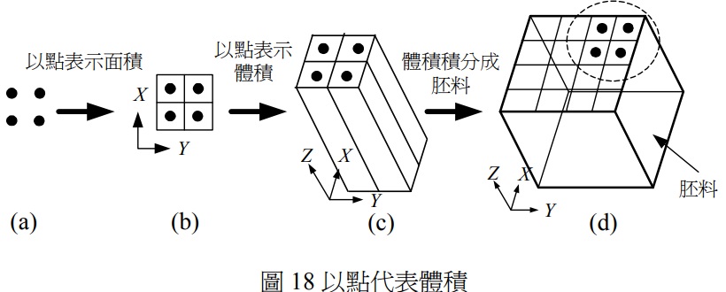
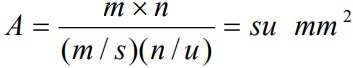
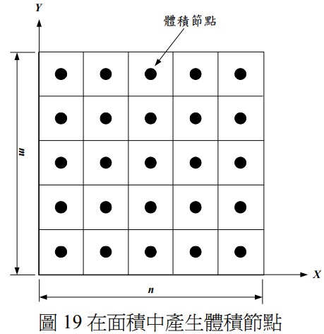
In an area of m X n, as shown in Fig. 19, one volume node is given every s and u, so the area A represented by one volume node can be obtained by the following equation
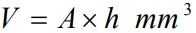
If the volume node drops by a distance h due to tool cutting during machining, the volume V removed can be obtained from the following equation.
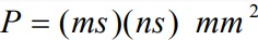
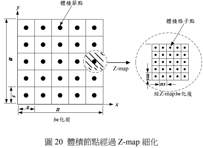
In order to remove the volume more accurately, this paper, in line with the Z-map method mentioned above, the above volume nodes, respectively, s and u divided by m s and ns once more, in order to find the nearby volume lattice points, as shown in Figure 20, at this time each volume lattice point represents the area P can be obtained from the following formula.
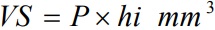
The volume VS of each volume lattice point removed when the distance of the drop in volume lattice points during machining due to tool cutting is hi can be obtained from the following equation.
After the Z-map method, the calculated removal volume is closer to the entity's Boolean calculation value. Then we simulate a tool on each CL point, calculate the total removal volume of the CL point, and use the total removal volume to find the cutting force of each CL point in the machining path in the order of the relational formula.
1. First calculate the volume of the remaining embodied material after roughing:
Since the roughing of this article is done using equal height machining, there are two types of toolpaths: straight and contoured. The approximate shape is first machined with a straight toolpath, and then the remaining volume of the edge is removed with a contoured toolpath, and the roughing of the volume is shown in Figure 21.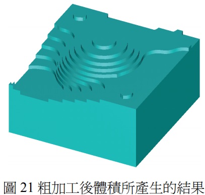
2. The volume removed from the CL point.
As shown in FIG. 22, each CL point on the path simulates a Boolean calculation in which the volume of a machining tool intersects with the above-mentioned lattice points of volume obtained through Z-map, and the removed volume of these lattice points is added together to obtain the total volume removed from this CL point, and the removed volume of all CL points is brought into the feed rate calculation formula in order.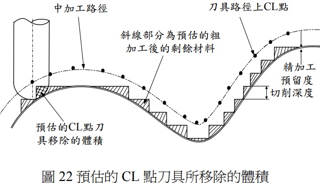
3-2 Principles for calculating process feed rates
In cutting mechanics, the cutting force is proportional to the volume of material removed by the tool. When the tool removes more material volume then the cutting force is greater, we can reduce the feed rate so that the cutting force is lower. When the tool removes less material volume and the cutting force is less, we can adjust the feed rate to make the cutting efficiency better. In this paper, in the adjustment of the feed rate of medium machining, the cutting force is first found and then the appropriate feed rate is adjusted by the size of the cutting force, where the relationship between the cutting force F and the chip removal volume V and the feed rate Vf can be deduced from the law of cutting force, and the deduction results are as follows.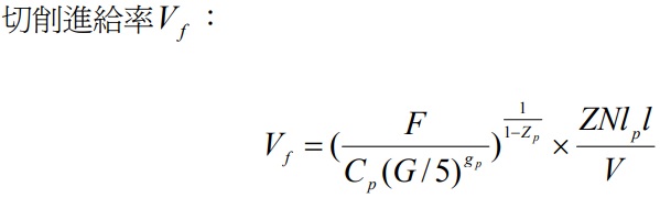
The cutting force required to cut the material per tooth of the tool F:
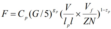
Among them
C p : Represents cutting cross-sectional area = 1mm 2 of cutting force.
G: Stands for the cut shape, which is the ratio of depth of cut to feed.
gp, zp: Represents the cutting force constant.
N : Represents spindle speed in rpm.
Z: Represents the number of teeth of the tool.
lp: Represents the length of the cutting path in mm.
l: Represents chip length in mm.
V: Represents chip removal volume in mm 3.
After deducing the relationship between cutting force and volume and feed rate, we input a fixed feed rate, which is used to calculate the cutting force at each CL point in the tool path with the size of the volume removed by the fixed feed rate, and substitute (10) to calculate the cutting force at each CL point under the fixed feed rate for subsequent adjustment of feed rate.
The basic idea of adjusting the feed rate is to vary the feed rate according to the volume removed during machining and the cutting force generated, so that the cutting force is kept within a reasonable range. When the cutting force is too large, the cutting force F is reduced, and the reduced cutting force is substituted in the formula (9) to obtain the adjusted feed rate Vf, so that the load on the tool in the process of machining will not be overloaded and affect the quality of the work.
3-3 Principles for calculating the feed rate for finishing
At this point, we hope that the removal rate of each cutting point is equal, so that the cutting force will not change too much, resulting in undercutting or broken tool. The following is a list of the principles for calculating the feed rate for different types of surfaces.
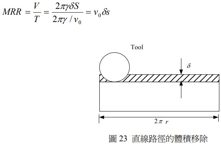
1. The feed rate of the straight path, as shown in Figure 23.
Volume removed during tool cutting V: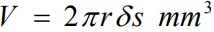
Where r : represents the cutting path distance parameter.
δ: Represents depth of cut in mm.
S: Stands for tool interval distance in mm.
Tool cutting time T (mim):
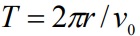
Where v0: represents the cutting speed of a straight line in mm/min.
From equations (11) and (12), the MRR (material removal rate) of tool cutting is collated.
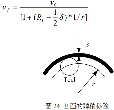
2. The cut surface is the feed rate of the concave surface, as shown in Figure 24.
The volume removal rate of its tool cutting MRR (mm 3 / mim).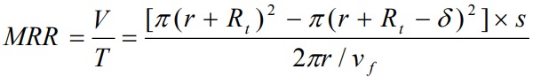
Where V: the volume removed, in mm 3 .
T: Tool cutting time, in mim.
R : represents the curvature radius of the cutting path.
δ: represents depth of cut in mm.
Rt: represents tool radius in mm.
S: represents the distance between the tools in mm.
Therefore, using the concept of equal volume removal rate, it can be deduced that the cutting speed vf (mm/min) of the concave surface is:
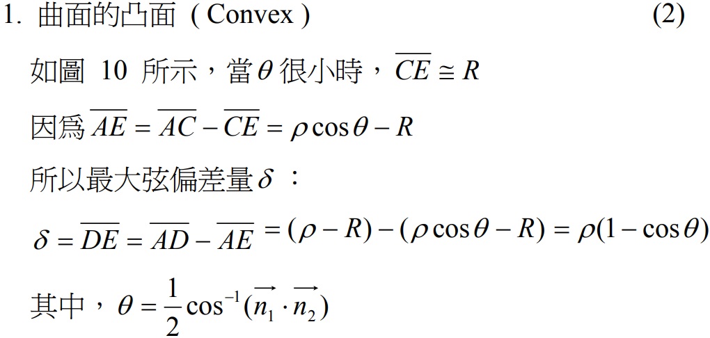
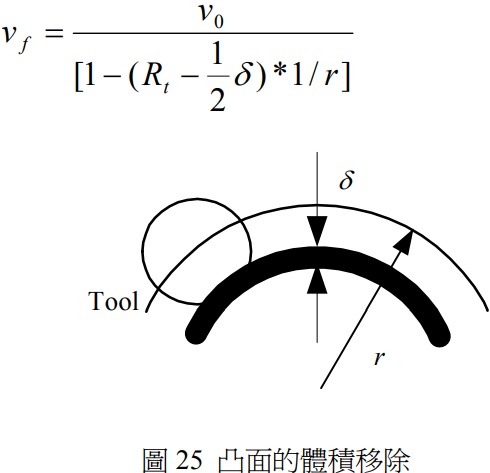
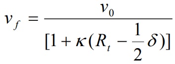
3. The feed rate of the cut surface is the convex surface, as shown in Figure 25.
Volume removal rate of its tool cutting MRR.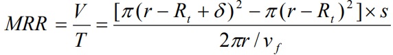
Where V: the volume removed
T: Tool cutting time
R : represents the curvature radius of the cutting path.
δ: represents depth of cut in mm.
Rt: represents tool radius in mm.
S: represents the distance between the tools in mm.
Thus using the concept of equal volume removal rate, the cutting speed vf (mm/min) of the convex surface can be deduced as:
From equations (15) and (17), the tool cutting feed rate Vf is collated:
Where Vf : represents the cutting tool feed rate in mm/min.
k : is the curvature, k is 1/r when concave, k is -1/r when convex.
3-4 Smoothing of the feed rate
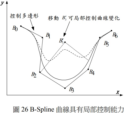
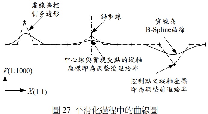
The rate of feed during machining or finishing may be too large due to the sudden change in the geometry of the cutting model, resulting in too large a change in the rate of feed at the two adjacent points, resulting in the machine's instantaneous large acceleration and deceleration, resulting in vibration phenomenon, so this paper uses the B-Spline curve to smooth this rate of feed.1. the designed curve will be contained within the raised housing of the control polygon, as shown in Figure 26.
2. has the characteristic of a local control curve, i.e., changing a control point will only affect the shape of the curve adjacent to this control point, as shown in Figure 26.
Next, we will present the detailed steps of how this article uses B-Spline curves to smooth out the feed rate.
1. find the control point of the B-Spline curve: take the straight line distance between two adjacent CL points projected in the X and Y planes as the horizontal coordinates of the control point of the B-Spline curve, and in equations (9) and (18), find the feed rate as the vertical coordinates of the control point of the B-Spline curve.
2. generate a B-Spline curve: pull a B-Spline curve from the control point obtained in the previous step, as shown in Figure 27.
3. Calculate the feed rate after B-Spline curve smoothing: Draw a vertical lead line at the control point, the vertical lead line must have an intersection with the B-Spline curve, and the vertical coordinates of the intersection are the feed rate after B-Spline curve smoothing, as shown in Figure 27.
IV. Implementation and verification of system functions
In this study, the ACIS geometric kernel is used as the core program to generate the workpiece embryos for the 3D solid model, and the Visual C++ programming language is used, the volume Boolean operation is used to find the volume of each processing point and the curvature of the processing point, and the adjusted feed rate is then used to find the adjusted feed rate by using the algorithm for medium and finishing machining proposed in the previous paper.
4-1 System Implementation Process
The detailed process of implementation of this system is as follows.1. Read the physical model of the workpiece embryo.
2. read the roughing NC machining code and remove the roughing material.
3. Showing the roughing profile: Remove the volume by reading the NC code and do the volume Boolean calculation between the volume generated by the roughing toolpath range and the original embryo to calculate the remaining volume after roughing.
4. Machining parameters to be machined in the setting: including workpiece material, tool diameter, machining tolerances, tool pitch, number of tool edges, feed rate, spindle rotation speed, tool safety height, and finishing allowance, etc.
5. Generate toolpaths for mid-machining: Take the grid points generated after Z-map and create a new curve through the point curve, which is the toolpath.
6. Adjusting the feed rate of machining: If the shape of the tool at each CL point is booleaned to the model volume, the corresponding volume of each CL point and the distance of each CL point can be obtained, and the cutting force at each CL point can be calculated by successively substituting the cutting force into the feed rate adjustment algorithm.
7. NC process code for processing in production.
8. Showing the shape after machining: In the tool path of machining, the remaining volume after machining can be calculated by using the volume of the tool shape and the volume of the rough machining at each CL point for boolean calculation.
9. Toolpath for finishing: Take the lattice point generated after Z-map and create a new curve through the point curve, which is the toolpath, with step length and tool spacing to find the appropriate finishing CL point.
10. Adjusting the feed rate for finishing: Find the curvature of each CL point on the cutting path of this CL point, and substitute the curvature into the algorithm for adjusting the feed rate in order to calculate the feed rate for each CL point, and use the B-Spline curve to smooth out the correction of the feed rate on the same cutting path to prevent the machine from vibrating due to excessive changes in feed rate.
11. Produce the NC process code for the finishing process.
In the input/output of data, first read the geometry data of the model workpiece, then set the machining parameters for machining and finishing, including workpiece material, tool length, tool diameter, toolpath interval, depth of cut, feed rate, spindle speed, tool safety height and machining reserve, etc. Finally, the machining toolpath and finishing toolpath are generated, and the feed rate suitable for machining is automatically adjusted and NC machining code is generated.
4-2 Example Verification
Figure 28 shows an example of the processing of a single surface solid model with the following steps.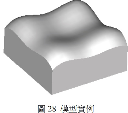
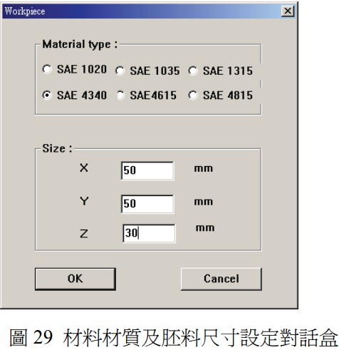
1. Set the processing material and embryo size, the workpiece size range is X: 50mm, Y: 50mm, Z: 30mm, the dialog box is shown in Figure 29.
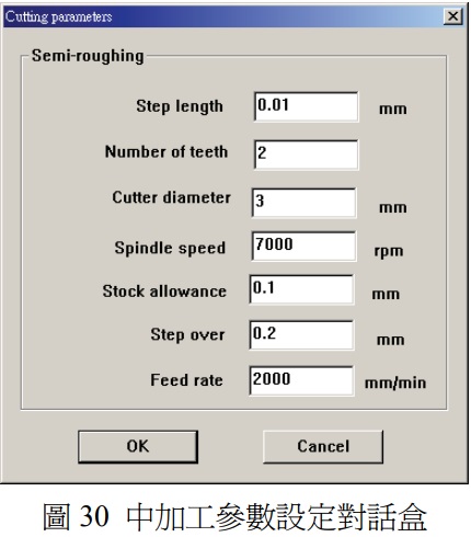
2. Set the parameters for machining, step length 0.01mm, number of blade teeth 2, finishing allowance 0.1mm, spindle speed 7000rpm, tool diameter 3mm, path pitch 0.2mm, initial feed rate 2500 mm/min, as shown in Figure 30.
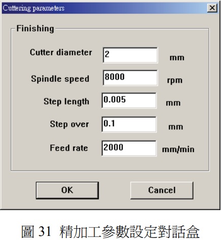
3. Set the parameters for finishing, step length 0.01mm, spindle speed 8000 rpm, tool diameter 2mm, initial feed rate 2000 mm/min, path spacing 0.1mm, dialog box, as shown in Figure 31.
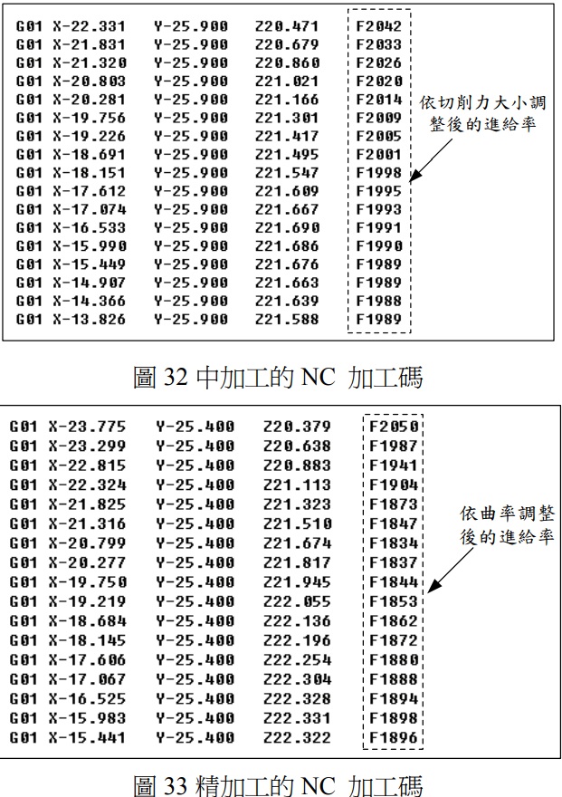
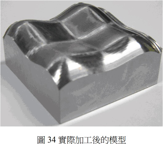
4. The final generation of NC machining codes for machining and finishing is shown in FIGS. 32 and 33.
5. The actual processed model, as shown in Figure 34.
4-3 Results and Discussion
It has been found that the feed rate adjustment algorithm is particularly suitable for software with no interpolation path function in the roughing path. When roughing no interpolation path function, cutting surface slope of the small area, the ladder embryo left behind is still too large, if directly in machining cutting, then the tool will be very large cutting force, and thus the phenomenon of vibration tool, some high-speed machining software with roughing interpolation path function, but its processing method is still unable to fully make the cutting force in machining to maintain a reasonable range, such as this paper proposed in the machining feed rate adjustment algorithm to calculate the true cutting volume of the concept of the feed rate, then the cutting force of the tool will be maintained within a reasonable range, which will improve the quality of processing.
V. Conclusion
In this study, an algorithm with adjustable feed rate is proposed to plan NC finishing toolpaths, and the proposed theory is validated using the ACIS geometric kernel. Its features are as follows.
1. During machining and finishing, the feed rate can be adjusted so that the load on the tool will not change too much and the tool will not be subjected to severe stress, so the tool is less likely to be damaged than usual.
2. when the cutting tool removes less material during machining, the tool feed rate can be faster, so machining time can be shortened.
3. The method of automatic feed rate adjustment for machining is very suitable for roughing machining without patching path function.
4. The concept of integration and Z-map theory are used to calculate the machining volume during machining, which is much faster than the general algorithm using solid volume Boolean.